
Lead Time Calculator
Lead Time Calculator
Break total lead time into its five components, see where the time actually goes, and get the safety stock and reorder point that result.
Lead time components (days)
Demand and variability
Where the time goes
| Component | Days | Share | Typical fix |
|---|
If you reduce lead time
| Reduction | New lead time | New safety stock | Units released |
|---|
Lead time is the total elapsed time from raising an order to having goods available to use or sell. It breaks into five components, each with a different owner and a different fix. The lead time calculator above splits the total, shows which component dominates, and converts the result into safety stock and a reorder point.
Treating lead time as a single number to negotiate downwards is why most reduction programmes generate activity without measurable improvement. The figure is an aggregate of five separate processes, and only two of them belong to your supplier.
Calculate lead time from its components
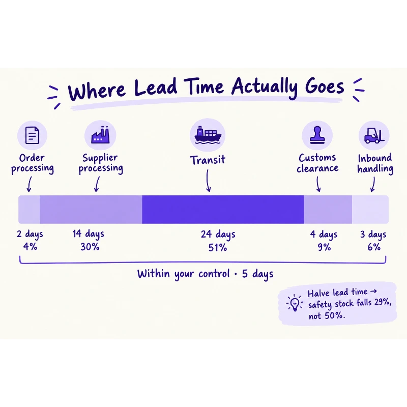
The lead time calculation is a sum rather than a formula. Add the elapsed days for each stage, then compare the result against what your system currently assumes.
| Component | Typical range | Owner | Usual fix |
|---|---|---|---|
| Order processing | 1 to 5 days | You | Electronic ordering, parallel approvals |
| Supplier processing | 7 to 30 days | Supplier | Rolling forecast visibility |
| Transit | 5 to 40 days | Carrier | Mode review, slot booking |
| Customs clearance | 1 to 15 days | Broker and you | Pre-arrival filing |
| Inbound handling | 1 to 7 days | You | Putaway priority, cross docking |
Two of the five sit entirely within your own organisation, which is worth establishing before any supplier conversation begins. Order processing and inbound handling frequently account for a week between them, and neither requires anyone else’s agreement to change.
Queue time is not process time
The sixth field in the tool captures something the standard five components miss: time spent waiting rather than being worked on.
A receiving operation processing six hundred lines a day but receiving nine hundred on a Monday has three hundred waiting on Tuesday, regardless of how efficiently each one is handled. That is a capacity problem wearing the costume of a process problem.
The distinction matters because process improvement does nothing for queue time. Only levelling the arrival pattern or adding capacity moves it, and organisations that misdiagnose it spend months optimising steps that were never the constraint.
Stated lead time and measured lead time
Most safety stock calculations use the figure held in ERP master data, frequently entered when the supplier relationship began and never revisited since.
Measured lead time, calculated from actual purchase order and goods receipt dates across twelve months, is commonly a third longer. Its variability is wider still than whatever figure is being used in the buffer calculation.
The symptom is stockouts occurring despite inventory the system reports as adequate. The cause is not the safety stock formula but its inputs, and correcting it requires a data extract rather than any investment.
The wider planning consequences are examined in our guide to supply chain planning.
Measuring lead time in a spreadsheet
Before buying anything, the measurement can be done in an afternoon with order and receipt dates exported from your system.
| What you want | Formula | Note |
|---|---|---|
| Calendar days per order | =B2-A2 | Format the result as a number, not a date |
| Working days per order | =NETWORKDAYS(A2,B2) | Excludes weekends automatically |
| Working days, custom weekend | =NETWORKDAYS.INTL(A2,B2,7) | For Friday and Saturday weekends |
| Average lead time | =AVERAGE(C2:C200) | The mean to use in planning |
| Variability | =STDEV.S(C2:C200) | Feeds the safety stock calculation |
| Planning figure at 95 percent | =PERCENTILE.INC(C2:C200,0.95) | What to promise against |
Run those formulas by supplier rather than across the whole dataset. An aggregate figure conceals the two or three relationships generating most of the variability, and those are exactly where attention belongs.
A lead-time calculator is only as good as the data behind it, so replace assumed figures with these measured ones before drawing conclusions from any buffer recommendation.
Why variability matters more than the average
A supplier reliably delivering in thirty days is easier to plan around than one averaging twenty-two but ranging from twelve to forty.
Safety stock is sized against variability rather than the mean. The second supplier has the better average and requires substantially more buffer, which means the apparently faster supplier is more expensive to work with once inventory cost is counted.
That is why the tool accepts lead time standard deviation separately, and why an improvement narrowing the range is frequently worth more than one shortening the average. Ask suppliers for consistency before asking for speed.
The square root relationship
Safety stock scales with the square root of lead time rather than in proportion to it.
| Lead time reduction | Safety stock reduction |
|---|---|
| 10% | About 5% |
| 25% | About 13% |
| 50% | About 29% |
| 64% | About 40% |
Halving lead time therefore removes roughly twenty-nine percent of required buffer, not fifty. The relationship is worth knowing before building a business case, because overstating the inventory release makes the whole proposal easy to dismiss. Understating it is equally unhelpful, since the real figure is usually large enough to justify the work on its own.
The sequence that produces results fastest
Attempting all five components simultaneously spreads effort thinly and shows little movement anywhere.
Start with customs clearance, because pre-arrival filing needs only workflow discipline and delivers within weeks. Move to order processing next, since it sits entirely within your control and usually hides several days in sequential approvals that could run in parallel.
Approach supplier processing third. It carries the largest opportunity and requires a forecast-sharing commitment that takes months to build credibility, so starting here means the first visible result arrives two quarters in and the initiative loses support before it lands.
Transit and queue time come last, because both generally require capital or a network decision rather than a process change. Running the lead time calculator after each intervention keeps the cumulative effect visible, which matters for sustaining support across a programme spanning several quarters.
The supplier conversation
Most supplier processing time exists because the supplier is scheduling reactively, and reactive scheduling costs them as much as it costs you.
A supplier receiving orders with no forward visibility cannot plan capacity, buy materials efficiently or level production. They hold their own buffer and price it into your unit cost, so you are already paying for the uncertainty.
Offering a rolling eight to twelve week forecast in exchange for a shorter committed lead time gives them something usable and costs you nothing you were not already forecasting internally. The forecasting discipline behind it is covered in AI forecasting and inventory planning.
One caution worth stating plainly. A shorter commitment agreed without any underlying operational change simply produces a number that is confidently wrong, and planning against it is worse than planning against the honest longer figure. Ask what specifically will be different before accepting a reduction.
Supplier reliability sits within the broader framework covered in managing supply chain risk, and the freight cost consequences of longer transit are examined in reducing transportation cost in logistics.
Where to begin
Knowing how to calculate lead time accurately is the prerequisite for every inventory decision downstream, because buffer, reorder point and promised delivery all rest on it.
Pull twelve months of order and receipt dates, calculate the real mean and standard deviation by supplier, and compare both against what your system currently holds. The gap is almost always larger than expected, and closing it costs nothing.
The lead time calculator above is built to accept those measured figures directly, which is why it takes demand and lead time variability as separate inputs rather than assuming either. For continuing coverage of lead times, carrier performance and planning practice, see our ongoing freight and operations reporting.
Frequently asked questions
How do you calculate lead time?
Add the elapsed days for each stage: order processing, supplier processing, transit, customs clearance and inbound handling. Alternatively measure it directly as the number of days between the purchase order date and the date goods became available to use.
What does 2-4 week lead time mean?
The supplier expects to deliver somewhere between 14 and 28 days from order confirmation, and the range reflects their own scheduling variability. Plan against the upper end, and confirm whether the clock starts at order placement or at payment, since the difference is often several days.
How do I calculate lead time in Excel?
Subtract the order date from the receipt date with =B2-A2 for calendar days, or use =NETWORKDAYS(A2,B2) for working days. Then apply =AVERAGE() for the mean and =STDEV.S() for variability, which is what safety stock calculations actually need.
How to calculate expected lead time?
Use the measured historical mean from actual order-to-receipt records rather than the figure stored in master data. For a planning figure with confidence built in, take the mean and add roughly 1.65 standard deviations to cover 95 percent of outcomes.